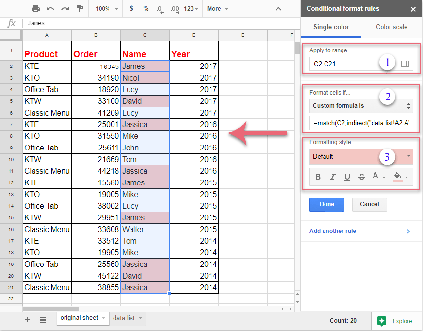
Google Sheets Conditional Formatting Based On Another Sheet - Web to format an entire row based on the value of one of the cells in that row: Web apply conditional formatting based on another sheet 1. =match (c2,indirect (data list!a2:a),0) |. From the file menu click format followed by. Select the range you want to format, for example, columns a:e. Select the range of cells to apply the conditional formatting to. You can use the custom formula function in google sheets to apply conditional formatting based on a cell value from another sheet. Select the cells you want to include in the. Web conditional formatting to highlight cells based on a list from another sheet in google sheets. Web conditional formatting is a helpful feature in google sheets that allows you to apply formatting to cells based on certain conditions.
From the file menu click format followed by. Conditional formatting from another sheet. =match (c2,indirect (data list!a2:a),0) |. Web to format an entire row based on the value of one of the cells in that row: Select the range of cells to apply the conditional formatting to. One way to use conditional formatting is to format cells. You can use the custom formula function in google sheets to apply conditional formatting based on a cell value from another sheet. On your computer, open a spreadsheet in google sheets. Select the range you want to format, for example, columns a:e. Select the cells you want to include in the.
One way to use conditional formatting is to format cells. =match (c2,indirect (data list!a2:a),0) |. Web to format an entire row based on the value of one of the cells in that row: Conditional formatting from another sheet. Select the range you want to format, for example, columns a:e. On your computer, open a spreadsheet in google sheets. Web apply conditional formatting based on another sheet 1. Select the cells you want to include in the. Select the range of cells to apply the conditional formatting to. You can use the custom formula function in google sheets to apply conditional formatting based on a cell value from another sheet.

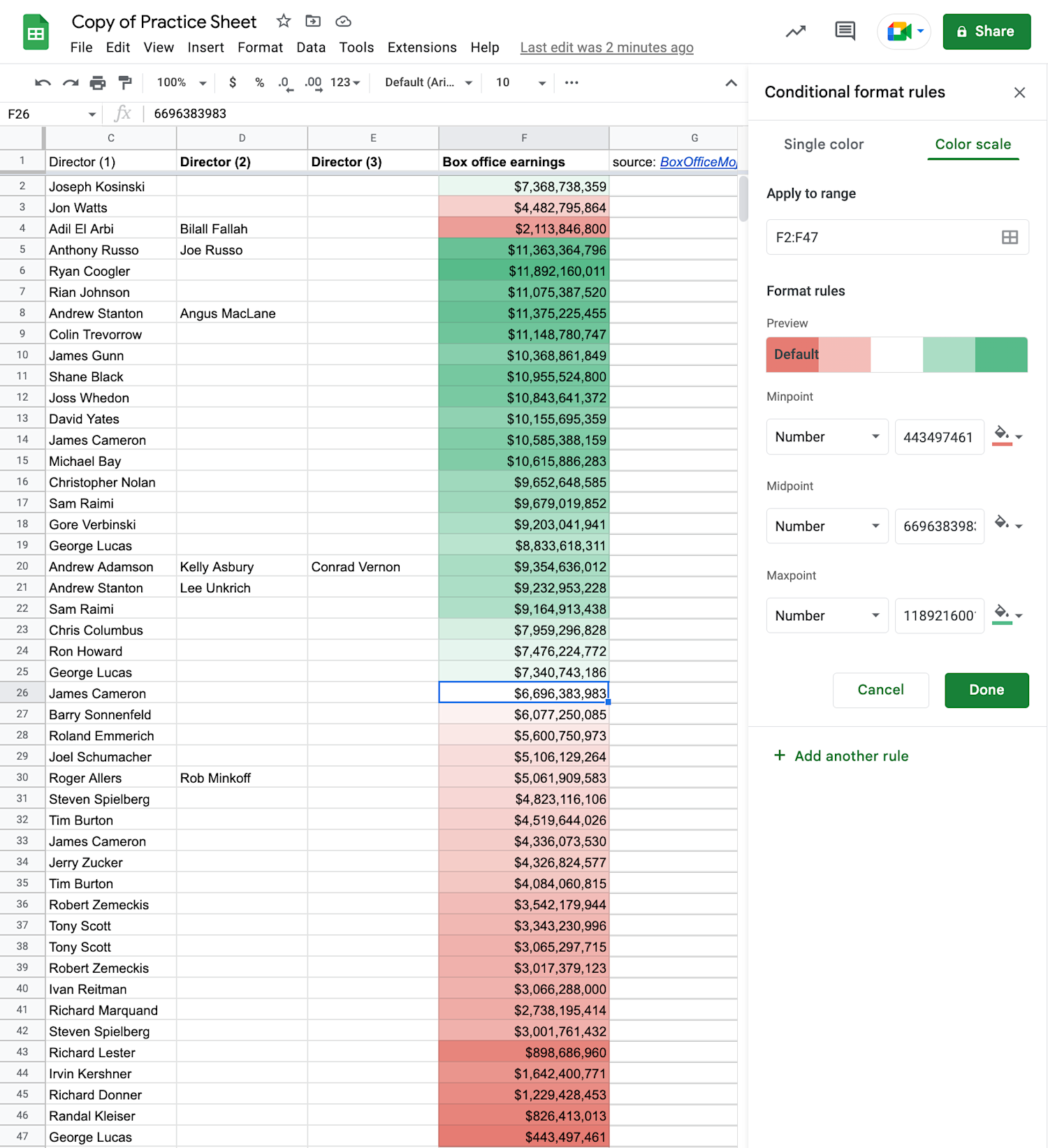
google sheets Conditional formatting with color scale for many rows
Select the cells you want to include in the. Web apply conditional formatting based on another sheet 1. Web conditional formatting is a helpful feature in google sheets that allows you to apply formatting to cells based on certain conditions. You can use the custom formula function in google sheets to apply conditional formatting based on a cell value from.

Conditional Formatting in Google Sheets Guide 2023 Coupler.io Blog
Web apply conditional formatting based on another sheet 1. From the file menu click format followed by. =match (c2,indirect (data list!a2:a),0) |. On your computer, open a spreadsheet in google sheets. Web conditional formatting to highlight cells based on a list from another sheet in google sheets.
How to conditional formatting based on another sheet in Google sheet?
One way to use conditional formatting is to format cells. =match (c2,indirect (data list!a2:a),0) |. Conditional formatting from another sheet. Web to format an entire row based on the value of one of the cells in that row: Web apply conditional formatting based on another sheet 1.
How to Use Google Sheets to Create Conditional Formatting Rules
From the file menu click format followed by. Web to format an entire row based on the value of one of the cells in that row: One way to use conditional formatting is to format cells. Select the cells you want to include in the. You can use the custom formula function in google sheets to apply conditional formatting based.
Use name in custom formatting excel boutiquepilot
Web to format an entire row based on the value of one of the cells in that row: One way to use conditional formatting is to format cells. =match (c2,indirect (data list!a2:a),0) |. Select the cells you want to include in the. Select the range of cells to apply the conditional formatting to.
How to Use Conditional Formatting in Google Sheets Coursera
Web conditional formatting to highlight cells based on a list from another sheet in google sheets. On your computer, open a spreadsheet in google sheets. Web conditional formatting is a helpful feature in google sheets that allows you to apply formatting to cells based on certain conditions. Web to format an entire row based on the value of one of.

Google Sheets Indirect Conditional Formatting Sablyan
Select the range you want to format, for example, columns a:e. On your computer, open a spreadsheet in google sheets. From the file menu click format followed by. =match (c2,indirect (data list!a2:a),0) |. Select the range of cells to apply the conditional formatting to.
How to Use Google Spreadsheet Conditional Formatting to Highlight
Web apply conditional formatting based on another sheet 1. From the file menu click format followed by. =match (c2,indirect (data list!a2:a),0) |. Select the cells you want to include in the. One way to use conditional formatting is to format cells.

Google Sheets Beginners Conditional Formatting (09) Yagisanatode
Select the range you want to format, for example, columns a:e. You can use the custom formula function in google sheets to apply conditional formatting based on a cell value from another sheet. From the file menu click format followed by. Conditional formatting from another sheet. Web conditional formatting to highlight cells based on a list from another sheet in.

Conditional Formatting in Google Sheets Guide 2023 Coupler.io Blog
On your computer, open a spreadsheet in google sheets. Web conditional formatting is a helpful feature in google sheets that allows you to apply formatting to cells based on certain conditions. Select the range of cells to apply the conditional formatting to. Conditional formatting from another sheet. From the file menu click format followed by.
You Can Use The Custom Formula Function In Google Sheets To Apply Conditional Formatting Based On A Cell Value From Another Sheet.
Web conditional formatting is a helpful feature in google sheets that allows you to apply formatting to cells based on certain conditions. From the file menu click format followed by. One way to use conditional formatting is to format cells. Web apply conditional formatting based on another sheet 1.
Select The Cells You Want To Include In The.
Conditional formatting from another sheet. Select the range you want to format, for example, columns a:e. On your computer, open a spreadsheet in google sheets. =match (c2,indirect (data list!a2:a),0) |.
Select The Range Of Cells To Apply The Conditional Formatting To.
Web to format an entire row based on the value of one of the cells in that row: Web conditional formatting to highlight cells based on a list from another sheet in google sheets.